Satcos

Classification techniques predict smaller set of discrete values as apposed to regression which predicts continuous values. One special case named Binary classification which involves just two classes. To understand internal workings of Logistic Regression algorithm lets use binary classification problem, which can be extended to multi-class easily.

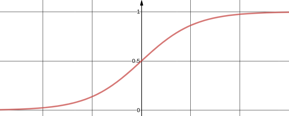
We need a function which maps any value of independent variable $x$ to dependent variable $y$ which ranges from 0 to 1. The values of $y$ are interpreted as probabilities of positive class. For example our problem involves classifying mails as Spam or Not Spam and we treat Spam as positive class, then $y$ represent probability of given input being a Spam. Sigmoid function is one suitable function which ranges from 0 to 1. Below figure shows Sigmoid function in single dimension, it can be easily extended to multiple dimensions. $y$ tends to 1 when $x$ tends to $\infty$ and $y$ tends to zero when $x$ tends to $-\infty$

$$y = {1 \over 1 + e^{-x}}$$ $$h_{\theta}(x) = g(\theta^{T} x) = {1 \over {1 + e^{-\theta^T x}}}$$

In $h_{\theta}(x)$ the subscript $\theta$ represent the function $h$ is parameterized by $\theta$, in optimization language $\theta$ is the free variable. For multi dimensional $x$, $\theta^{T} x$ can be conveniently expanded. $\theta_0$ is explicitly included to account for intercept.

$$\theta^{T} x = \theta_0 + \sum_{j=1}^n {\theta_j x_j}$$ $$P(y=1|x;\theta) = h_{\theta}(x)$$ $$P(y=0|x;\theta) = 1 - h_{\theta}(x)$$

Now to fit $\theta$ Above two equation can be rewritten as

$$P(y|x;\theta) = (h_{\theta}(x))^y (1 - h_{\theta}(x))^{1-y}$$

Assuming m training examples, writing the likelihood function $$L(\theta) = \prod_{i=1}^m {p(y^{(i)}|x^{(i)};\theta)} $$ $$L(\theta) = \prod_{i=1}^m {(h_{\theta}(x^{(i)}))^{y^{(i)}} (1 - h_{\theta}(x^{(i)}))^{1-y^{(i)}}} $$ Log likelihood $$l(\theta) = \sum_{i=1}^m {y^{(i)} log h_{\theta}(x^{(i)}) + (1-y^{(i)}) log(1 - h_{\theta}(x^{(i)}))} $$ The $\theta$ that maximizes the likelihood function is the solution.

In order to get more clarity lets workout these steps in excel. You can get the sample dataset from here. It has 400 rows and 4 columns admit, gre. gpa and rank. admit is the outcome variable and all other are continuous independent variables. Take a glance at some of the important variables in the below screenshoot.

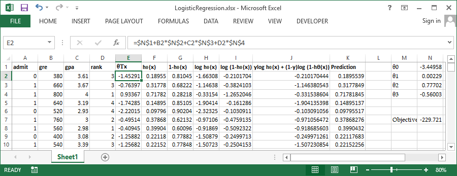
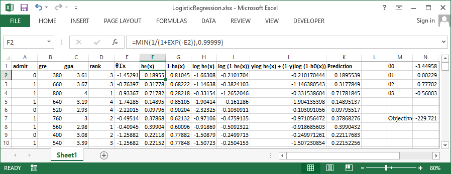
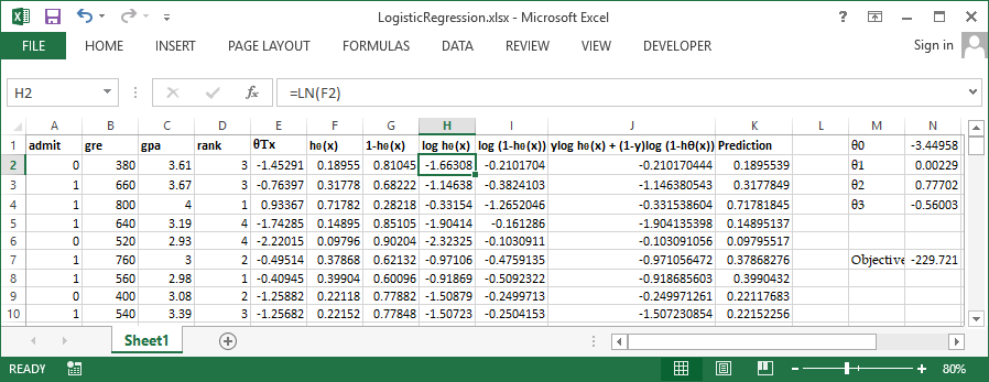
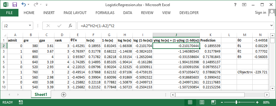
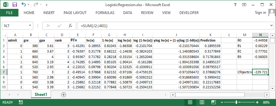
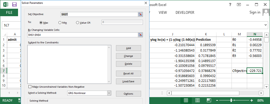
Use inbuild solver available in excel to perform the optimization, Set cell N7 (Sum of column J) to be maximized by varying $\theta0$ to $\theta3$ Let's try the same problem in R and verify our output